Demandlib Electricity Model Example

This notebook demonstrates how to use Demandlib electricity model to electricity loads for multiple buildings.

Imports

Import required libraries and set visualization defaults.

import os

import pandas as pd
import matplotlib.pyplot as plt

from entise.core.generator import Generator
from entise.constants import Types

Load Data

We load building parameters from objects.csv and simulation data from the data folder.

# Load data
cwd = "."  # notebook runs inside examples/electricity_demandlib

objects = pd.read_csv(os.path.join(cwd, "objects.csv"))

data = {}
common_data_folder = "../common_data"

for file in os.listdir(os.path.join(cwd, common_data_folder)):
    if file.endswith(".csv"):
        name = file.split(".")[0]
        data[name] = pd.read_csv(
            os.path.join(cwd, common_data_folder, file),
            parse_dates=True,
        )

print("Loaded data keys:", list(data.keys()))

Loaded data keys: ['validation_weather', 'weather']
📋 Loaded 10 objects

Instantiate and Configure Model

Initialize the time series generator and configure it with building objects.

gen = Generator()
gen.add_objects(objects)

summary, df = gen.generate(data, workers=1)

100%|██████████| 10/10 [00:02<00:00,  3.51it/s]

Results Summary

Below is a summary of the annual electricity demands (in kWh/a) and peak loads (W).

print("Summary:")
summary_kwh = (summary / 1000).round(0).astype(int)
summary_kwh.rename(columns=lambda x: x.replace("[W]", "[kW]").replace("[Wh]", "[kWh]"), inplace=True)
print(summary_kwh.to_string())

Summary:
    electricity:demand[kWh]  electricity:load_max[kW]
1                      3002                         1
2                      4004                         1
3                         0                         0
4                     50013                        13
5                     20016                         5
6                      2012                         1
7                    204530                        54
8                    201030                        53
9                    204536                        54
10                   278032                        74

Preparation of Data

# Prepare data
building_id = objects["id"].iloc[0]
res = df.get(building_id)

df = res[Types.ELECTRICITY]
df.index = pd.to_datetime(df.index, utc=True)

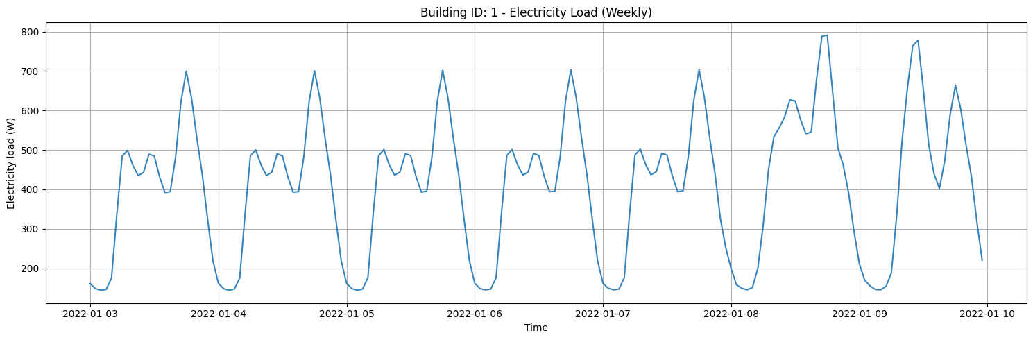
Visualization of Results

Visualize weekly electricity loads for a selected building.

def plot_weekly_profile():
        # Pick the first full week starting Monday (or fallback: first 7 days)
        start = df.index.min().normalize()
        start = start + pd.Timedelta(days=(7 - start.weekday()) % 7)
        end = start + pd.Timedelta(days=7)

        s_week = df.loc[(df.index >= start) & (df.index < end)]

        fig, ax = plt.subplots(figsize=(15, 5))
        ax.plot(s_week.index, s_week.values, alpha=0.9)
        ax.set_title(f"Building ID: {building_id} - Electricity Load (Weekly)")
        ax.set_xlabel("Time")
        ax.set_ylabel("Electricity load (W)")
        ax.grid(True)
        plt.tight_layout()
        plt.show()

plot_weekly_profile()

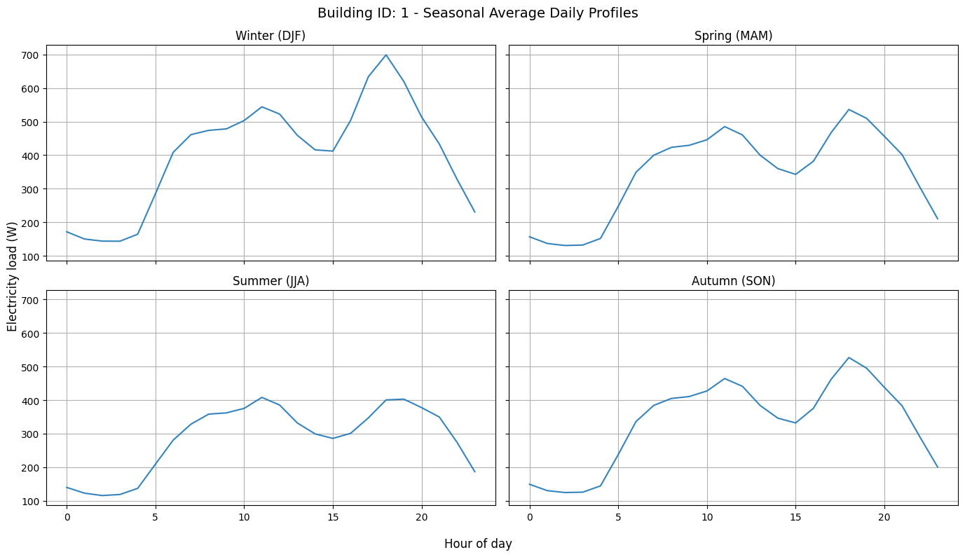
Seasonal Electricity Loads

Next, we visualize the electricity loads for different seasons

def plot_seasonal_subplots():
        df_tmp = df.copy()
        df_tmp.columns = ["load"]
        df_tmp["month"] = df_tmp.index.month
        df_tmp["hour"] = df_tmp.index.hour

        # Map month → season (no helper defs)
        df_tmp["season"] = "Autumn (SON)"
        df_tmp.loc[df_tmp["month"].isin([12, 1, 2]), "season"] = "Winter (DJF)"
        df_tmp.loc[df_tmp["month"].isin([3, 4, 5]), "season"] = "Spring (MAM)"
        df_tmp.loc[df_tmp["month"].isin([6, 7, 8]), "season"] = "Summer (JJA)"
        df_tmp.loc[df_tmp["month"].isin([9, 10, 11]), "season"] = "Autumn (SON)"

        prof = df_tmp.groupby(["season", "hour"])["load"].mean().reset_index()

        fig, axes = plt.subplots(2, 2, figsize=(14, 8), sharex=True, sharey=True)
        axes = axes.flatten()

        season_order = ["Winter (DJF)", "Spring (MAM)", "Summer (JJA)", "Autumn (SON)"]

        for i, season in enumerate(season_order):
            ax = axes[i]
            df_season = prof[prof["season"] == season]
            ax.plot(df_season["hour"], df_season["load"], alpha=0.9)
            ax.set_title(season)
            ax.grid(True)

        fig.suptitle(f"Building ID: {building_id} - Seasonal Average Daily Profiles", fontsize=14)
        fig.supxlabel("Hour of day")
        fig.supylabel("Electricity load (W)")
        plt.tight_layout()
        plt.show()

plot_seasonal_subplots()