Demandlib Heating Model Example

This notebook demonstrates how to use Demandlib space heating model to simulate heating loads for multiple buildings.

Imports

Import required libraries and set visualization defaults.

import os

import pandas as pd
import matplotlib.pyplot as plt

from entise.core.generator import Generator
from entise.constants import Types
from entise.constants import Columns as Cols

Load Data

We load building parameters from objects.csv and simulation data from the data folder.

# Load data
cwd = "."  # notebook runs inside examples/heat_demandlib

objects = pd.read_csv(os.path.join(cwd, "objects.csv"))

data = {}
common_data_folder = "../common_data"

for file in os.listdir(os.path.join(cwd, common_data_folder)):
    if file.endswith(".csv"):
        name = file.split(".")[0]
        data[name] = pd.read_csv(
            os.path.join(cwd, common_data_folder, file),
            parse_dates=True,
        )

print("Loaded data keys:", list(data.keys()))

Loaded data keys: ['validation_weather', 'weather']

Instantiate and Configure Model

Initialize the time series generator and configure it with building objects.

gen = Generator()
gen.add_objects(objects)

summary, df = gen.generate(data, workers=1)

100%|██████████| 10/10 [00:01<00:00,  6.43it/s]

Results Summary

Below is a summary of the annual heating demands (in kWh/a) and peak loads (W).

print("Summary:")
summary_kwh = (summary / 1000).round(0).astype(int)
summary_kwh.rename(columns=lambda x: x.replace("[W]", "[kW]").replace("[Wh]", "[kWh]"), inplace=True)
print(summary_kwh.to_string())

Summary:
    heating:demand[kWh]  heating:load_max[kW]
1                  5578                     2
2                  1701                     1
3                  1073                     0
4                 11792                     5
5                  3487                     1
6                 28220                    12
7                 23140                    10
8                  5180                     2
9                 23180                    10
10                10614                     4

Preparation of Data

# Define the building ID to process and visualize
building_id = summary.index[0]  # Change index to visualize different buildings

# Visualize results for the processed building
# Note: We're using the same building_id as defined above
building_data = df[building_id][Types.HEATING]

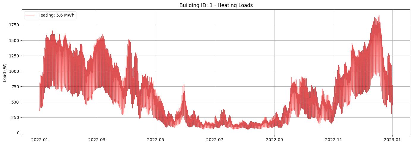
Visualization of Results

Visualize heatingloads for a selected building.

def plot_heating_loads():
    """Heating and Cooling Loads"""
    fig, ax = plt.subplots(figsize=(14, 5))
    heating_MWh = summary.loc[building_id, "heating:demand[Wh]"] / 1e6
    (line1,) = ax.plot(
        pd.to_datetime(building_data.index, utc=True),
        building_data["heating:load[W]"],
        label=f"Heating: {heating_MWh:.1f} MWh",
        color="tab:red",
        alpha=0.8,
    )
    # Create the combined legend in the upper left corner
    ax.set_ylabel("Load (W)")
    ax.set_title(f"Building ID: {building_id} - Heating Loads")
    ax.legend()
    ax.grid(True)
    plt.tight_layout()
    plt.show()

plot_heating_loads()

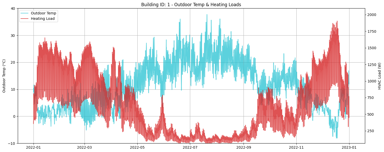
Outdoor Temperature with Heating Loads

Next, we visualize the outdoor temperature alongside the heating loads to see how they correlate.

def plot_outdoor_temp_with_loads():
    """Outdoor Temperature with Heating & Cooling Loads"""
    fig, ax1 = plt.subplots(figsize=(15, 6))

    # Plot outdoor temperature on left y-axis
    air_temp = data["weather"][f"{Cols.TEMP_AIR}@2m"]
    ax1.plot(
        pd.to_datetime(building_data.index, utc=True), air_temp, label="Outdoor Temp", color="tab:cyan", alpha=0.7
    )

    ax1.set_ylabel("Outdoor Temp (°C)")
    ax1.set_ylim(air_temp.min().round() - 2, air_temp.max().round() + 2)

    # Create second y-axis for loads
    ax2 = ax1.twinx()
    ax2.plot(
        pd.to_datetime(building_data.index, utc=True),
        building_data["heating:load[W]"],
        label="Heating Load",
        color="tab:red",
        alpha=0.8,
    )
    ax2.set_ylabel("HVAC Load (W)")
    ax2.set_ylim(
        building_data["heating:load[W]"].min() * 1.1,
        building_data["heating:load[W]"].max() * 1.1,
    )

    # Combine legends from both axes
    lines1, labels1 = ax1.get_legend_handles_labels()
    lines2, labels2 = ax2.get_legend_handles_labels()
    ax1.legend(lines1 + lines2, labels1 + labels2, loc="upper left")

    ax1.set_title(f"Building ID: {building_id} - Outdoor Temp & Heating Loads")
    ax1.grid(True)
    fig.tight_layout()
    plt.show()

plot_outdoor_temp_with_loads()