Occupancy: PHT
This notebook demonstrates how to infere the occupancy schedule of a dwelling based on the Page-Hinkley Test (PHT) of its electricity demand, following the implementation by Becker et al. (2017).
Imports
Import required libraries and set visualization defaults.
import logging
import os
import matplotlib.pyplot as plt
import numpy as np
import pandas as pd
from entise.constants import Types, Objects as O, SEP
from entise.constants.columns import Columns
from entise.core.generator import Generator
%matplotlib inline
Load Data
We load building parameters from objects.csv and simulation data from the data folder.
# Load data
cwd = f""  # Current working directory: change if your kernel is not running in the same folder
objects = pd.read_csv(os.path.join(cwd, "objects.csv"))
data = {}
common_data_folder = "../common_data"
for file in os.listdir(os.path.join(cwd, common_data_folder)):
    if file.endswith(".csv"):
        name = file.split(".")[0]
        data[name] = pd.read_csv(os.path.join(os.path.join(cwd, common_data_folder, file)), parse_dates=True)

data_folder = "data"
for file in os.listdir(os.path.join(cwd, data_folder)):
    if file.endswith(".csv"):
        name = file.split(".")[0]
        data[name] = pd.read_csv(os.path.join(os.path.join(cwd, data_folder, file)), parse_dates=True)
print("Loaded data keys:", list(data.keys()))
Loaded data keys: ['validation_weather', 'weather', 'demand_1_occupants', 'demand_2_occupants', 'demand_4_occupants']
Instantiate and Configure Model
Initialize the time series generator and configure it with building objects.
gen = Generator(logging_level=logging.WARNING)
gen.add_objects(objects)
Run the Simulation
Generate sequential occupancy detection for each object.
summary, dfs = gen.generate(data, workers=1)
100%|██████████| 12/12 [00:06<00:00, 1.74it/s]
Results Summary
Below is a summary of the average detected occupancy for a whole year.
print("Summary:")
print(summary)
Summary occupancy:
    occupancy:average_occupancy
1                          0.26
2                          0.56
3                          0.61
4                          0.16
5                          0.27
6                          0.26
7                          0.26
8                          0.22
9                          0.49
10                         0.23
11                         0.40
12                         0.33
Visualization of Results
Visualize the Electricity demand and Occupancy schedule for a certain day of the year. As well as monthly occupancy percentage.
Prepare data for visualization
# Prepare data for visualization
OBJECT_CONFIGS = {
        1: {"color": "tab:cyan", "texture": "x", "legend": "ID 1 (Detection Threshold: 0.3, Without NS)"},
        2: {"color": "tab:orange", "texture": "..", "legend": "ID 2 (Detection Threshold: 0.3, With NS)"},
        3: {"color": "tab:green", "texture": "*", "legend": "ID 3 (Detection Threshold: 0.7, With NS)"},
    }

#Pick a day of the year
day_of_year=182 # half of the year

#Generate 1 dataframe per object and filter by selected day
df_1=dfs[1].copy()

df_1[Types.OCCUPANCY]=df_1[Types.OCCUPANCY].loc[df_1[Types.OCCUPANCY].index.dayofyear==day_of_year]
df_1[Types.ELECTRICITY][Columns.DATETIME]=pd.to_datetime(df_1[Types.ELECTRICITY][Columns.DATETIME],
                                                         utc=True).dt.tz_convert("Europe/Berlin")
df_1[Types.ELECTRICITY]=df_1[Types.ELECTRICITY].set_index(Columns.DATETIME)
df_1[Types.ELECTRICITY]=df_1[Types.ELECTRICITY].loc[df_1[Types.ELECTRICITY].index.dayofyear==day_of_year]

df_2=dfs[2].copy()

df_2[Types.OCCUPANCY]=df_2[Types.OCCUPANCY].loc[df_2[Types.OCCUPANCY].index.dayofyear==day_of_year]
df_2[Types.ELECTRICITY][Columns.DATETIME]=pd.to_datetime(df_2[Types.ELECTRICITY][Columns.DATETIME],
                                                         utc=True).dt.tz_convert("Europe/Berlin")
df_2[Types.ELECTRICITY]=df_2[Types.ELECTRICITY].set_index(Columns.DATETIME)
df_2[Types.ELECTRICITY]=df_2[Types.ELECTRICITY].loc[df_2[Types.ELECTRICITY].index.dayofyear==day_of_year]

df_3=dfs[3].copy()

df_3[Types.OCCUPANCY]=df_3[Types.OCCUPANCY].loc[df_3[Types.OCCUPANCY].index.dayofyear==day_of_year]
df_3[Types.ELECTRICITY][Columns.DATETIME]=pd.to_datetime(df_3[Types.ELECTRICITY][Columns.DATETIME],
                                                         utc=True).dt.tz_convert("Europe/Berlin")
df_3[Types.ELECTRICITY]=df_3[Types.ELECTRICITY].set_index(Columns.DATETIME)
df_3[Types.ELECTRICITY]=df_3[Types.ELECTRICITY].loc[df_3[Types.ELECTRICITY].index.dayofyear==day_of_year]
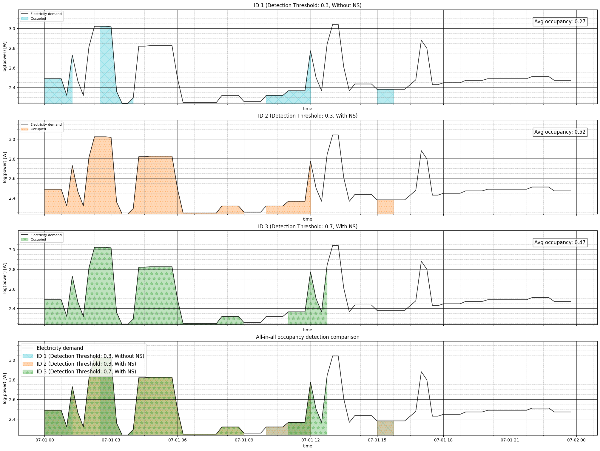
Plot 1: Daily Comparison for Different Occupancy Detection Configurations
Shows how different detection thresholds and the use of the nightly schedule detection algorithm yields different occupancy schedules for a specific day of the year.
fig, axs = plt.subplots(nrows=4, ncols=1, figsize=(20, 15), sharex=True, constrained_layout=True)

def style_ax(ax, title, ymin):
    ax.set_title(title, fontsize=12)
    ax.set_xlabel("time", fontsize=10)
    ax.set_ylabel("log(power) [W]", fontsize=10)
    ax.set_ylim(bottom=ymin)
    ax.minorticks_on()
    ax.grid(which="major", linestyle="-", linewidth=0.5, color="black")
    ax.grid(which="minor", linestyle=":", linewidth=0.5, color="gray")

def plot_object_data(ax, df, cfg, show_legend=True):
    """Plot electricity demand and occupancy for a single object"""
    log_power = np.log10(df[Types.ELECTRICITY][Columns.POWER])
    occupancy_col = f"{Types.OCCUPANCY}{SEP}{Columns.OCCUPANCY}"

    # Plot electricity demand
    ax.plot(df[Types.OCCUPANCY].index, log_power, color="black", alpha=0.8)

    # Fill occupied periods
    ax.fill_between(
        df[Types.OCCUPANCY].index, log_power,
        where=df[Types.OCCUPANCY][occupancy_col] == 1,
        color=cfg["color"], hatch=cfg["texture"], alpha=0.3
    )

    # Style and legend
    style_ax(ax, cfg["legend"], log_power.min())
    if show_legend:
        ax.legend(["Electricity demand", "Occupied"], fontsize=8, loc="upper left")

    # Add average occupancy text
    avg_occ = df[Types.OCCUPANCY][occupancy_col].mean().round(2)
    ax.text(0.98, 0.9, f"Avg occupancy: {avg_occ}",
            transform=ax.transAxes, ha="right", va="top",
            bbox=dict(facecolor="white", alpha=0.7), fontsize=12)

# Plot individual objects (IDs 1-3)
dfs_list = [df_1, df_2, df_3]
for i, (df, obj_id) in enumerate(zip(dfs_list, [1, 2, 3])):
    plot_object_data(axs[i], df, OBJECT_CONFIGS[obj_id])

# All-in-all comparison plot
ax = axs[3]
ax.plot(df_1[Types.OCCUPANCY].index,
        np.log10(df_1[Types.ELECTRICITY][Columns.POWER]),
        color="black", alpha=0.8)

# Fill between for all objects
occupancy_col = f"{Types.OCCUPANCY}{SEP}{Columns.OCCUPANCY}"
for df, obj_id in zip(dfs_list, [1, 2, 3]):
    ax.fill_between(
        df[Types.OCCUPANCY].index,
        np.log10(df[Types.ELECTRICITY][Columns.POWER]),
        where=df[Types.OCCUPANCY][occupancy_col] == 1,
        color=OBJECT_CONFIGS[obj_id]["color"],
        hatch=OBJECT_CONFIGS[obj_id]["texture"],
        alpha=0.3
    )

style_ax(ax, "All-in-all occupancy detection comparison",
         np.log10(df_1[Types.ELECTRICITY][Columns.POWER]).min())
ax.legend(["Electricity demand"] + [OBJECT_CONFIGS[i]["legend"] for i in [1, 2, 3]],
          fontsize=12, loc="upper left")

plt.show()
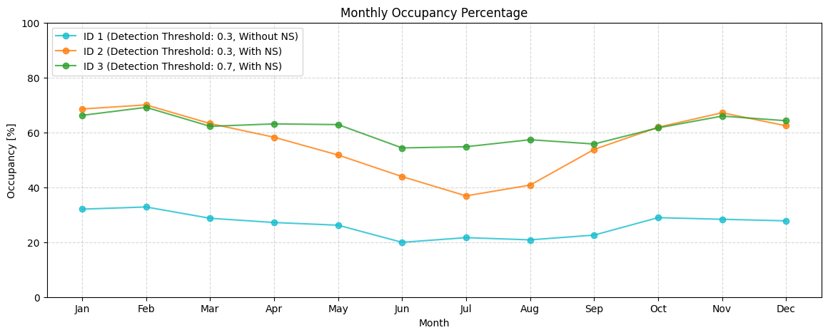
Plot 2: All in All Monthly Average
Shows the monthly percentage of occupancy for the 3 different objects.
fig, ax = plt.subplots(figsize=(14, 5))

for obj_id, cfg in OBJECT_CONFIGS.items():

    occ = dfs[obj_id][Types.OCCUPANCY]

    occ.index = pd.to_datetime(occ.index,utc=True).tz_convert("Europe/Berlin")

    monthly_occ = (
        occ[f"{Types.OCCUPANCY}{SEP}{Columns.OCCUPANCY}"]
        .groupby(occ.index.month)
        .mean()
        .mul(100)
        .sort_index()
    )

    ax.plot(
        monthly_occ.index,
        monthly_occ.values,
        marker="o",
        label=cfg["legend"],
        color=cfg["color"],
        alpha=0.8,
    )

ax.set_title("Monthly Occupancy Percentage", fontsize=12)
ax.set_xlabel("Month")
ax.set_ylabel("Occupancy [%]")
ax.set_ylim(0, 100)
ax.grid(True, which="both", linestyle="--", alpha=0.5)
ax.set_xticks(range(1, 13))
ax.set_xticklabels(
    ["Jan", "Feb", "Mar", "Apr", "May", "Jun",
     "Jul", "Aug", "Sep", "Oct", "Nov", "Dec"]
)
ax.legend(fontsize=10, loc="upper left")

plt.show()
Next Steps
You can further:
Explore the effect on different seasons of the year.
Apply higher or lower detection thresholds, baseline offsets or lambda values,
or different nightly schedule configurations.
Explore the effect that electricity demands with different time resolution have on the detected occupancy.